ACS Advocacy Workshops
ACS Climate Change Advocacy Workshop

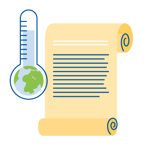
The purpose of this free, online, and interactive workshop is for participants to learn how to effectively advocate for climate change action on the federal level. The workshop includes modules covering an overview of climate change science, some of its impacts on society and the environment, as well as mitigation, adaptation, and resiliency strategies. It also explores how the U.S. government is involved with climate change action. Importantly, participants will learn about different ways to communicate about climate change with various audiences, from those who are champions of climate change action to those who are less receptive to climate change, while always moving toward a shared common goal. This program aligns with ACS' ongoing engagement with policymakers on Capitol Hill in support of science, engineering, innovation, and chemical stewardship.
Module topics include:
- The science of climate change
- Climate change and society
- Climate change and the U.S. government
- Climate change communications
- Conclusions and Advocacy Activities
ACS Chemistry Advocacy Workshop

The ACS Chemistry Advocacy Program is designed to help ACS members passionate about science and chemistry advocacy maximize Society resources through in-person workshops or this on-demand course.
This workshop is online and includes four modules covering skills, resources, logistics, and communication for the purposes of advocating for chemistry on the federal level. Participants will learn to successfully plan and execute advocacy activities, as well as have an opportunity to network and build a community with others passionate about science advocacy and ACS. This program aligns with ACS' ongoing engagement with policymakers on Capitol Hill in support of science, engineering, innovation, and chemical stewardship.
Module topics include:
- Introduction to chemistry advocacy
- Chemistry advocacy within the U.S. government
- Advocating for chemistry with Congress
- Chemistry communication for advocates
;void(0);)